How-To: Working with Evaluations

The evals package reads solved PyPSA networks, computes energy-system statistics, and renders interactive visualisations. This guide explains the architecture, shows you how to register new views, and walks through the pypsa.statistics API that underpins every chart.

Architecture: Model–View–Component

The evaluation pipeline follows a pattern that maps cleanly onto three concepts:

Role	Implementation	Responsibility
Model	`pypsa.NetworkCollection`	Holds one solved `pypsa.Network` per planning year
View	`evals.views.*`	Queries statistics and prepares data for a specific chart
Component	`evals.plots.*`	Renders a Plotly figure from the prepared data

NetworkCollection ──► view_balance_electricity()
                           │
                           ├─ collect_myopic_statistics("supply", …)
                           ├─ collect_myopic_statistics("withdrawal", …)
                           ├─ rename / aggregate via config.categories
                           └─ Exporter ──► ESMBarChart.plot()
                                                │
                                          HTML + JSON output

Model — `pypsa.NetworkCollection`

A NetworkCollection is a thin dictionary wrapper mapping planning year (int) to a pypsa.Network. Use read_networks to load one from a result directory:

from evals.fileio import read_networks

nc = read_networks("results/my_scenario")
# nc.networks == {2030: <Network>, 2050: <Network>}

read_networks also patches each network with ESMStatistics so that n.statistics.<method>() is available on every loaded network.

Views — `evals.views`

A view is a plain function with the signature:

def view_<name>(result_path: Path, nc: NetworkCollection, config: dict) -> None:
    ...

It collects one or more statistics, applies category renaming from the config, constructs an Exporter, and calls exporter.export(). All 23 built-in views are importable from evals.views:

from evals.views import view_balance_electricity, view_capacity_electricity_production

Components — `evals.plots`

Each view delegates rendering to one of four chart classes:

Class	Best for
`ESMBarChart`	Single-location stacked bar (supply/demand, capacities)
`ESMGroupedBarChart`	Faceted bars — one subplot per `bus_carrier` (heat systems, fuel groups)
`ESMTimeSeriesChart`	Hourly stacked area / line charts
`SankeyChart`	Full system energy-flow diagram

The chart class used by each view is declared in config.default.toml under the chart key and can be overridden per view (see Configuration).

Configuration

Config layers

View parameters live in two TOML files that are deep-merged at runtime (last wins):

evals/config.default.toml   ← shipped defaults (do not edit)
        ↓
evals/config.override.toml  ← your local overrides (create this file)

Each view has its own section:

[view_balance_electricity]
name   = "Electricity Energy Balance"
unit   = "TWh_el"
chart  = "ESMBarChart"          # which plot class to use
cutoff = 0.1                    # values below this (in unit) are dropped

[view_balance_electricity.categories]
"onwind"     = "Wind Power"     # internal carrier name → nice name
"offwind-ac" = "Wind Power"     # multiple carriers can map to the same nice name
"solar"      = "Solar Power"

How deep-merge works

The merge uses pydantic.v1.utils.deep_update, which recurses into nested dicts but replaces everything else wholesale. The practical rules are:

Value type	Merge behaviour	Example
Dict (e.g. `categories`)	Keys are merged. Override adds new keys and overwrites existing ones; keys not present in the override are kept from default.	Adding `"new carrier" = "Nice Name"` in override leaves all default mappings intact.
List (e.g. `legend_order`, `bus_carrier`)	The override list replaces the default list entirely. Partial updates are not possible — you must repeat every item you want to keep.	Setting `legend_order = ["Wind", "Solar"]` discards all other entries from the default.
Scalar (e.g. `cutoff`, `name`, `chart`)	The override value replaces the default value.	`cutoff = 0.5` overrides the default `0.1`.

# config.override.toml — adding one category and tightening the cutoff
[view_balance_electricity]
cutoff = 0.5                          # replaces the scalar 0.1 from default

[view_balance_electricity.categories]
"allam gas" = "Thermal Powerplant"   # merged into the default categories dict

Key config keys

Name	Type	Description	Default
`name`	`str`	Plot title shown in the chart header	required
`unit`	`str`	Y-axis label	required
`file_name`	`str`	Output filename template; supports `{location}` and `{year}` placeholders	required
`chart`	`str`	Plot class to instantiate — one of `"ESMBarChart"`, `"ESMGroupedBarChart"`, `"ESMTimeSeriesChart"`, `"SankeyChart"`	required
`cutoff`	`float`	Drop rows whose absolute value is below this threshold (in the view's unit)	`0.1`
`bus_carrier`	`str \\| list[str]`	Filter statistics to buses with this carrier. Accepts a single string or a list.	`""` (all)
`storage_links`	`list[str]`	Carriers to exclude from the production/demand sides and reclassify as storage	`[]`
`legend_order`	`list[str]`	Display order of category labels in the legend, from bottom to top	`[]`
`categories`	`dict[str, str]`	Maps raw carrier strings to display (nice) names. Multiple carriers can share the same display name — they are summed after renaming.	`{}`
`checks`	`list[str]`	Consistency checks to run after export. Currently supports `"balances_almost_zero"`.	`[]`
`exports`	`list[str]`	Additional export formats beyond HTML. Currently supports `"csv"`.	`[]`

Switching chart types

The chart class is just a string in config — you can swap ESMBarChart for ESMGroupedBarChart (or vice versa) in your override file without touching any Python:

# config.override.toml
[view_balance_electricity]
chart = "ESMGroupedBarChart"   # split by bus_carrier instead of stacking all in one

This works whenever the data shape produced by the view is compatible with the target chart. Bar-type charts (ESMBarChart, ESMGroupedBarChart) share the same data contract; switching between them is always safe.

Registering a new view

Write the view function in the appropriate module under evals/views/:

# evals/views/myviews.py
from pathlib import Path
from pypsa import NetworkCollection
from evals.statistic import collect_myopic_statistics
from evals.fileio import Exporter, read_views_config

def view_my_metric(result_path: Path, nc: NetworkCollection, config: dict) -> None:
    stat = collect_myopic_statistics(nc, "supply", bus_carrier="H2")
    exporter = Exporter([stat], config["view"])
    exporter.export(result_path)

Export it from evals/views/__init__.py:

from evals.views.myviews import view_my_metric
__all__ = [..., "view_my_metric"]

Add a config section to config.default.toml (or config.override.toml):

[view_my_metric]
name      = "My Metric"
unit      = "TWh"
chart     = "ESMBarChart"
cutoff    = 0.1
file_name = "my_metric_{location}"

[view_my_metric.categories]
"H2 Electrolysis" = "Electrolysis"

Run it via the CLI:

pixi run evals "results/my_scenario" --views view_my_metric

Understanding `pypsa.statistics`

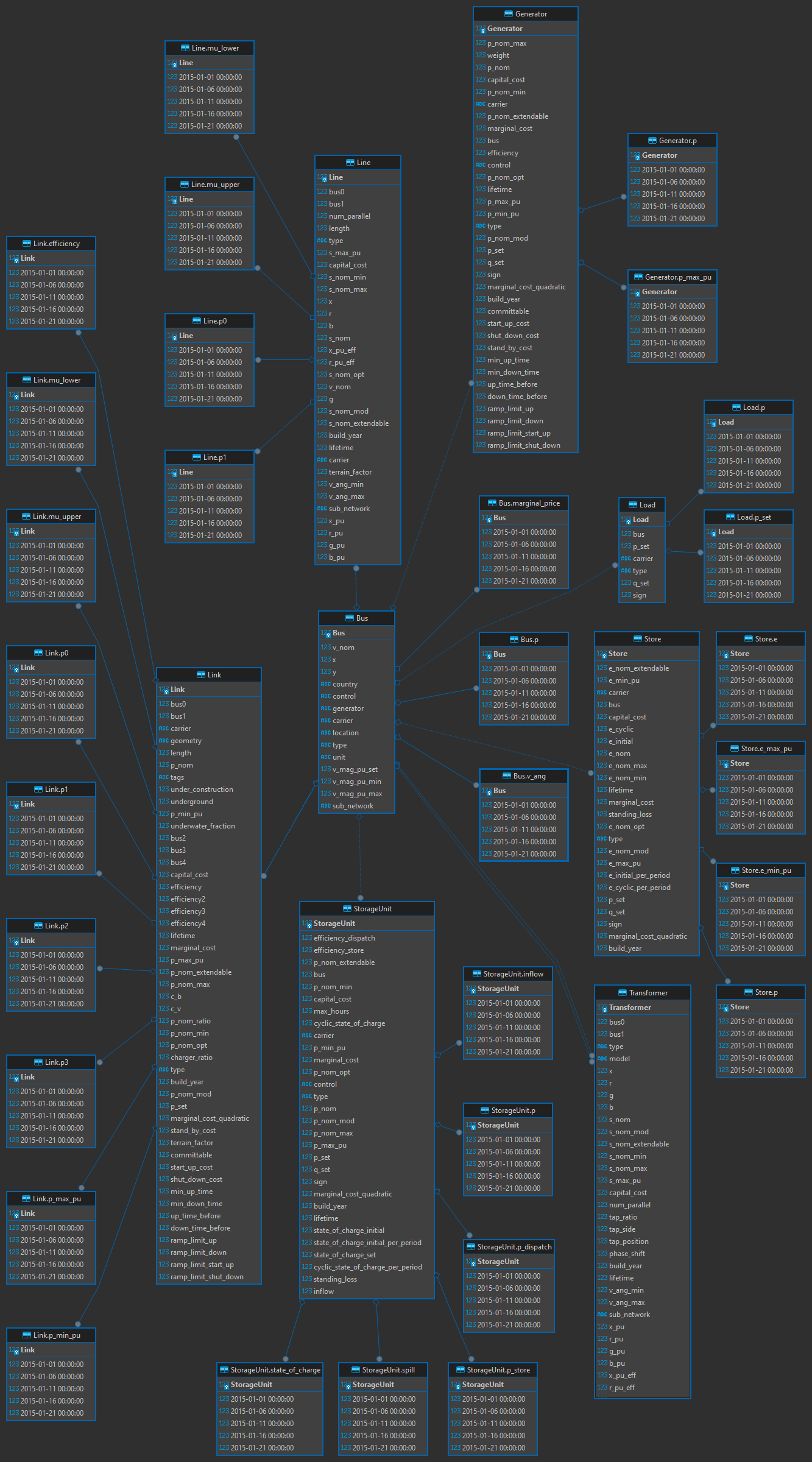
The network data model

A solved PyPSA network stores its components (Generators, Links, Lines, Stores, Loads …) as static DataFrames and their time-dependent results as Panel DataFrames (n.pnl("Generator")["p"]). Every component is connected to one or more buses. Each bus has a carrier attribute that identifies the energy carrier it represents (e.g. "AC", "H2", "gas", "urban central heat").

PyPSA post-network data model

The key attributes used by statistics are:

Name	Type	Location	Description
`carrier`	`str`	Component static DataFrame (e.g. `n.generators`)	Technology identifier, e.g. `"onwind"`, `"H2 Electrolysis"`
`bus` / `bus0` / `bus1`	`str`	Component static DataFrame	Name(s) of the connected bus. One-port components use `bus`; branch components use `bus0` and `bus1`.
`carrier`	`str`	`n.buses`	Energy carrier of the bus, e.g. `"AC"`, `"H2"`, `"gas"`
`location`	`str`	`n.buses`	Geographic region of the bus, e.g. `"AT"`, `"DE"`

The `groupby` argument — step by step

n.statistics.supply(groupby=["location", "carrier", "bus_carrier"]) groups component contributions into a labelled MultiIndex Series. Here is what happens internally:

Step 1 — Iterate components. PyPSA visits each component type (Generator, Link, …). For every component instance it evaluates each grouper function, producing a label.

Step 2 — Evaluate groupers.

Name	Type	Source	Example value
`location`	`str`	Bus `location` attribute (custom grouper, avoids EU nodes for branch components)	`"AT"`
`carrier`	`str`	Component `carrier` column	`"onwind"`
`bus_carrier`	`str`	Carrier of the connected bus	`"AC"`
`unit`	`str`	Statistic unit metadata	`"MWh"`

Step 3 — Group and aggregate. All component instances that share the same label tuple are summed together.

Step 4 — Build the MultiIndex. The result is a pd.Series indexed by a MultiIndex with one level per grouper:

location  carrier         bus_carrier
AT        onwind          AC            12 500 000.0    # MWh
          solar           AC             5 200 000.0
          H2 Electrolysis H2             3 100 000.0
DE        onwind          AC            20 300 000.0
dtype: float64

Step 5 — Year prefix (added by collect_myopic_statistics). When iterating over multiple planning years, a year level is prepended as the outermost index:

year  location  carrier         bus_carrier
2030  AT        onwind          AC            12 500 000.0
                H2 Electrolysis H2             1 400 000.0
2050  AT        onwind          AC            18 700 000.0
                H2 Electrolysis H2             8 200 000.0

Step 6 — Category mapping. The categories table in the view config is a many-to-one rename dictionary. rename_aggregate replaces each carrier label with its nice name and sums rows that now share the same tuple:

year  location  carrier     bus_carrier
2030  AT        Wind Power  AC            12 500 000.0   # onwind → Wind Power
2050  AT        Wind Power  AC            18 700 000.0

Worked example: navigating the foreign-key chain

Every grouper value is resolved by following PyPSA's implicit foreign-key relationships between DataFrames. Taking the bus_carrier and location groupers applied to Links as a concrete example shows exactly how the four DataFrames connect.

1 — Time-series column labels are component names.

n.links_t.p stores dispatch results with snapshots as rows and Link names as columns. Those column labels are the primary key of the static n.links table:

n.links_t.p.columns
# Index(['AT onwind-1', 'AT solar-1', 'DE gas CHP-1'], dtype='object', name='Link')

2 — Link names look up rows in n.links.

Each column label is a row in n.links. The bus0 column holds the name of the connected input bus — a foreign key into the n.buses index:

n.links.loc[n.links_t.p.columns, ["carrier", "bus0"]]
#               carrier          bus0
# AT onwind-1    onwind     AT AC bus
# AT solar-1      solar     AT AC bus
# DE gas CHP-1      gas    DE gas bus

3 — Bus names look up rows in n.buses.

n.buses["carrier"] maps each bus name to an energy carrier; n.buses["location"] maps it to a geographic region. These are the raw values that the bus_carrier and location groupers will produce:

n.buses.loc[["AT AC bus", "DE gas bus"], ["carrier", "location"]]
#            carrier location
# AT AC bus       AC       AT
# DE gas bus     gas       DE

4 — .map() chains the two lookups into a grouper Series.

The statistics machinery calls Series.map() to resolve each link name to its final label in a single vectorised step. For bus_carrier:

n.links["bus0"].map(n.buses["carrier"]).loc[n.links_t.p.columns]
# AT onwind-1     AC
# AT solar-1      AC
# DE gas CHP-1    gas
# Name: carrier, dtype: object

For location, substitute n.buses["location"]:

n.links["bus0"].map(n.buses["location"]).loc[n.links_t.p.columns]
# AT onwind-1     AT
# AT solar-1      AT
# DE gas CHP-1    DE
# Name: location, dtype: object

One such Series is computed per groupby entry. PyPSA combines them into a MultiIndex, aggregates the snapshot-weighted dispatch values within each group, and produces the labelled result from Steps 3–5 above.

Custom groupers registered by evals

The evals module registers three additional named groupers at import time:

Name	Type	Function	Description
`location`	`str`	[`get_location`][evals.statistic.get_location]	Maps bus → region; for branch components, prefers the non-EU endpoint
`bus0`	`str`	[`get_location_from_name_at_port`][evals.statistic.get_location_from_name_at_port] (port 0)	Extracts the location from the bus0 name string
`bus1`	`str`	[`get_location_from_name_at_port`][evals.statistic.get_location_from_name_at_port] (port 1)	Extracts the location from the bus1 name string

These names can be used directly in the groupby list:

n.statistics.transmission(groupby=["bus0", "bus1", "carrier"])

`collect_myopic_statistics`

collect_myopic_statistics is the primary entry point used inside view functions. It handles the multi-year iteration and ensures a consistent index structure across all statistics:

from evals.statistic import collect_myopic_statistics

stat = collect_myopic_statistics(
    nc,
    "supply",                    # positional: name of the n.statistics method to call
    bus_carrier=["AC", "H2"],   # keyword argument forwarded to the statistics method
    aggregate_components="sum", # merge Lines and Links into one row (default)
    drop_unit=True,             # store unit in attrs, drop from index (default)
)

The groupby default when calling a standard StatisticsAccessor method is: ["location", "carrier", "bus_carrier", "unit"].

Available `pypsa.statistics` methods

These methods are available on every n.statistics accessor (provided by StatisticsAccessor):

Method	Unit	Description
`supply`	MWh	Energy delivered to a bus by a component. Covers Generators dispatching, Links converting, Stores discharging. Always positive.
`withdrawal`	MWh	Energy drawn from a bus by a component. Covers Loads, Links consuming at input port, Stores charging. Always positive (sign convention: withdrawal is positive withdrawal).
`transmission`	MWh	Net energy transported by branch components (Line, Link used as transmission). Bidirectional.
`energy_balance`	MWh	Multi-port balance for each component port; tracks input and output at every port of a Link separately (useful for conversion-chain accounting).
`optimal_capacity`	MW	Post-optimisation capacity (p_nom_opt). The main capacity result.
`installed_capacity`	MW	Pre-existing capacity (`p_nom` with `p_nom_extendable=False`).
`expanded_capacity`	MW	New capacity added by the optimiser (`optimal - installed`).
`capex`	currency	Annualised capital expenditure for all capacities (installed + expanded).
`installed_capex`	currency	Annualised CAPEX for pre-existing capacities only.
`expanded_capex`	currency	Annualised CAPEX for newly built capacities only.
`fom`	currency	Fixed operations and maintenance cost (proportional to optimal capacity).
`opex`	currency	Variable (fuel + marginal cost) operational expenditure.
`overnight_cost`	currency	Total overnight investment cost (not annualised).
`system_cost`	currency	Total system cost = annualised CAPEX + OPEX.
`curtailment`	MWh	Energy that could have been generated but was curtailed by the optimiser. Relevant for VRE generators.
`capacity_factor`	—	Ratio of actual generation to the theoretical maximum (p_nom × hours). Ranges 0–1.
`revenue`	currency	Revenue earned at shadow prices of connected buses.
`market_value`	currency/MWh	Revenue per unit of energy; indicates how well a technology captures peak prices.
`prices`	currency/MWh	Average marginal price per bus (dual variable of the nodal balance constraint), weighted by supply.

In addition, ESMStatistics (the subclass registered by evals) provides:

Method	Unit	Description
`trade_energy`	MWh	Energy exchanged between locations. Scope can be `"foreign"` (cross-country), `"domestic"` (same country, different regions), or `"local"` (same location, different carrier). Positive = import, negative = export.
`trade_capacity`	MW	Transmission capacity between locations for the given scope and bus carrier.

Code examples

Querying annual supply by technology

from evals.fileio import read_networks
from evals.statistic import collect_myopic_statistics

nc = read_networks("results/my_scenario")

supply = collect_myopic_statistics(
    nc,
    "supply",
    bus_carrier="AC",              # electricity buses only
)

print(supply)
# year  location  carrier  bus_carrier
# 2030  AT        onwind   AC           12 500 000.0
#                 solar    AC            5 200 000.0
# 2050  AT        onwind   AC           18 700 000.0
# dtype: float64

Filtering by multiple bus carriers

balance = collect_myopic_statistics(
    nc,
    "supply",
    bus_carrier=["H2", "gas"],   # hydrogen and methane buses
    groupby=["location", "carrier", "bus_carrier"],
)

Querying optimal capacity

capacities = collect_myopic_statistics(
    nc,
    "optimal_capacity",
    bus_carrier="H2",
)
# Unit stored in attrs: capacities.attrs["unit"] == "MW"

Peak flows with `aggregate_time="max"`

For time-dependent statistics (transmission, trade_energy, energy_balance) the result is a DataFrame with snapshots as columns when aggregate_time=False. Passing aggregate_time="max" collapses the time axis by taking the maximum across all snapshots — giving you peak instantaneous flows rather than annual sums.

Note

"max" skips snapshot weighting (no multiplication by snapshot_weightings). The result is the raw peak value in the native unit (MW for power, MWh for single-snapshot energy amounts when the resolution is 1 h).

# Peak hydrogen pipeline flow — useful for infrastructure sizing
peak_h2_flow = collect_myopic_statistics(
    nc,
    "transmission",
    bus_carrier="H2",
    groupby=["bus0", "bus1", "carrier"],
    aggregate_time="max",        # peak snapshot value instead of annual sum
)

print(peak_h2_flow)
# year  bus0  bus1  carrier
# 2030  AT    DE    H2 pipeline    450.0   # MW
# 2050  AT    DE    H2 pipeline    820.0

# Peak electricity import into Austria
peak_import = collect_myopic_statistics(
    nc,
    "trade_energy",
    scope="foreign",
    direction="import",
    bus_carrier="AC",
    aggregate_time="max",        # peak hour instead of yearly total
)

# Yearly sum (default) for comparison
annual_wind = collect_myopic_statistics(nc, "supply", bus_carrier="AC")
# aggregate_time defaults to "sum" inside collect_myopic_statistics

Keeping the time axis

Pass aggregate_time=False to get a DataFrame with snapshots as columns. This is what the view_timeseries_* views use internally:

ts = collect_myopic_statistics(
    nc,
    "supply",
    bus_carrier="AC",
    aggregate_time=False,        # returns DataFrame: index=MultiIndex, columns=snapshots
)
# ts.columns.name == "snapshots"

Views reference

The table below lists all built-in views, their default chart component, and a short description.

Switching components

The chart component is configured via the chart key in config.override.toml. Swapping between ESMBarChart and ESMGroupedBarChart is always safe because both accept the same data layout — use ESMGroupedBarChart when you want the data split into facets by bus_carrier, and ESMBarChart when a single stacked panel is enough. ESMTimeSeriesChart and SankeyChart have a different data contract and cannot be swapped with the bar-chart classes.

Balances

View function	Default component	Description
`view_balance_electricity`	`ESMBarChart`	Annual electricity supply and demand, split by technology and trade flows
`view_balance_carbon`	`ESMBarChart`	Net CO₂ balance: emissions (positive) vs. capture/sequestration (negative)
`view_balance_heat`	`ESMGroupedBarChart`	Heat supply and demand per heat system (urban central, urban decentral, rural)
`view_balance_hydrogen`	`ESMBarChart`	Hydrogen supply and demand, including trade and storage
`view_balance_methane`	`ESMBarChart`	Methane supply and demand across gas, biogas and industry buses
`view_balance_biomass`	`ESMBarChart`	Solid biomass supply and consumption across all conversion routes
`view_balance_fuels`	`ESMGroupedBarChart`	Primary fuel balances (oil, coal, solid biomass, waste, methanol, ammonia, uranium) grouped by carrier family

Time series

View function	Default component	Description
`view_timeseries_electricity`	`ESMTimeSeriesChart`	Hourly electricity production and demand for a selected year
`view_timeseries_hydrogen`	`ESMTimeSeriesChart`	Hourly hydrogen production and demand for a selected year
`view_timeseries_methane`	`ESMTimeSeriesChart`	Hourly methane production and demand for a selected year
`view_timeseries_carbon`	`ESMTimeSeriesChart`	Hourly CO₂ emissions and capturing for a selected year

Capacities

View function	Default component	Description
`view_capacity_electricity_production`	`ESMBarChart`	Optimal generation capacity on AC/low-voltage buses
`view_capacity_electricity_demand`	`ESMBarChart`	Optimal electricity-consuming capacity (electrolysers, heat pumps, compressors, …)
`view_capacity_electricity_storage`	`ESMBarChart`	Electricity storage volumes (PHS, batteries, EV fleet) in TWh
`view_capacity_gas_storage`	`ESMBarChart`	Gas storage volumes (methane and hydrogen stores) in TWh
`view_capacity_hydrogen_production`	`ESMBarChart`	Optimal hydrogen production capacity by technology
`view_capacity_heat_production`	`ESMGroupedBarChart`	Heat production capacity per heat system type
`view_capacity_gas_production`	`ESMBarChart`	Optimal methane production capacity (SNG, biogas, imports, …)

Demand

View function	Default component	Description
`view_demand_heat_total`	`ESMBarChart`	Total primary energy consumed for heat production, grouped by input carrier
`view_demand_heat_system`	`ESMGroupedBarChart`	Primary energy per heat system type (urban central, urban decentral, rural), grouped by input carrier
`view_demand_fed_total`	`ESMBarChart`	Final energy demand aggregated across all sectors
`view_demand_fed_sectoral`	`ESMGroupedBarChart`	Final energy demand split by sector (Transport, Industry, Agriculture, HH & Services)

Energy flow

View function	Default component	Description
`view_sankey`	`SankeyChart`	Full system energy-flow Sankey from primary energy through conversion to final demand, with pie charts for primary energy mix and FED breakdown